Mixture models with *mixglm* • mixglm

mixglm is an R package for fitting mixture models. This vignette documents its use.

Installation

The package mixglm uses NIMBLE which requires a compiler such as Rtools.exe. For installation instructions see: NIMBLE.

To install the development version of the mixglm package from GitHub use:

# install.packages("remotes")
remotes::install_github("adamklimes/mixglm")

Introduction

mixglm uses a Bayesian framework via NIMBLE to fit mixtures of regressions. It provides flexibility in the specification of these regressions allowing their mean, precision, and probability to be dependent on up to multiple predictors. It supports normal, beta, gamma, or negative binomial distributed response variables.

Mixtures of regressions can be used for various purposes. Mixture models can be used as a semi-parametric way for modelling variables with an unknown distribution (McLachlan & Peel, 2000). They can be used in cluster analyses, or in resilience modelling (ecology) for parametrization of stability landscapes.

The mixglm package provides tools for exploration of results such as computations and visualizations of mixtures. While these tools are usable for all above mentioned purposes, they are described in the terminology of resilience modelling in this vignette.

mixglm for resilience modelling

Resilience is often illustrated using a ball rolling on a curve, where the ball represents a system which rolls into a valley representing a stable state. Due to a disturbance or internal stochasticity, the ball can be pushed up from the stable state. Resilience can be then defined as either local or non-local stability of the ball on the curve. If the slopes of the valley are steep, the system is locally stable and highly resilient (so called engineering resilience). If the nearest hill (local maximum of the curve, a tipping point) is far from the system position, then the system is stable also non-locally and has high ecological resilience (see review Dakos & Kéfi, 2022).

This stability curve can change its shape along external predictors creating a so-called stability landscape (see Klimeš et al., 2024). Mixture of regressions can be used to parametrize this stability landscape. From it, stability curves for predictor values of interest can be explored and the position of instances of a system (e.g. observed ecological systems) along these curves can be evaluated. mixglm offers tools for such purposes, ranging from stability landscape calculation and visualization, depiction of specified stability curves, to calculation of several metrics of ecological resilience.

Fitting mixture models using mixglm

In mixglm, it is possible to fit mixtures with a predefined number of components that have normal, beta, gamma, or negative binomial distribution (all components have the same distribution). For each component, its mean, precision, and probability within the mixture can be defined as being dependent on predictors which can differ between components (and also between mean, precision, probability sub-model). In the following we present a step-by-step guide for fitting a mixture model using mixglm.

Package set-up and data preparation

We start by loading the mixglm package and generating data for the example. We generate two example variables, one representing a precipitation gradient and the other being a proxy for ecosystem state - such as vegetation height. To fully illustrate the functionality of mixglm, vegetation height will have a multimodal distribution for a part of the precipitation gradient representing two alternative states.

library(mixglm)
#> Loading required package: nimble
#> nimble version 1.3.0 is loaded.
#> For more information on NIMBLE and a User Manual,
#> please visit https://R-nimble.org.
#> 
#> Note for advanced users who have written their own MCMC samplers:
#>   As of version 0.13.0, NIMBLE's protocol for handling posterior
#>   predictive nodes has changed in a way that could affect user-defined
#>   samplers in some situations. Please see Section 15.5.1 of the User Manual.
#> 
#> Attaching package: 'nimble'
#> The following object is masked from 'package:stats':
#> 
#>     simulate
#> The following object is masked from 'package:base':
#> 
#>     declare

st <- function(x, y = x) (x - mean(y)) / sd(y)  # standardization function

set.seed(10)
n <- 300
state <- rbinom(n, 1, 0.5)
precip <- runif(n, c(200, 600)[state + 1], c(1600, 2000)[state + 1])
vegHeight <- rnorm(n, c(1000, 2000)[state + 1], 100)
precipSt <- st(precip)
vegHeightSt <- st(vegHeight)
dat <- data.frame(vegHeight, precip, vegHeightSt, precipSt)

plot(vegHeight ~ precip, data = dat, ylab = "Vegetation height (cm)")

We generated an auxiliary latent variable state which describes which of the two ecosystem states any particular observation belongs. We assumed vegetation height to be normally distributed with parameters depending on this state.

Fitting the mixture model

To fit a mixture model, we must specify three sub-models. The first sub-model (stateValModels) specifies the mean values of mixture components, the second (statePrecModels) their precision, and the third (stateProbModels) their probability within the mixture. Each of them is specified by a formula with predictors on the right side.

In resilience modelling, we typically do not have a priori reasons to differentiate predictors between mixture components nor between sub-models. This means that mean, precision, and probability of each component can change along each predictor (see below; but one might want to limit the flexibility to facilitate the fit, especially with modest datasets - e.g. by constraining the precision to be constant: statePrecModels = ~ 1).

We also need to specify the number of components in the mixture (numStates). In resilience modelling, this number should at least correspond to the number of hypothesized alternative stable states. However, multiple components can together represent one stable state, therefore it is advisable to select a higher number of components. The number of components can be determined using the Watanabe-Akaike information criterion (WAIC; Watanabe, 2013) by running the model with different numbers and selecting the model with the lowest WAIC.

In our example, we will use just two components for simplicity. We also use standardized response variable and predictor to mean 0 and standard deviation 1. Standardization is recommended since it facilitates model fitting (especially finding starting values for the sampler and specification of informative priors if desired). We also specify the error distribution as gaussian in our case.

mod <- mixglm(
  stateValModels = vegHeightSt ~ precipSt,
  statePrecModels = ~ precipSt,
  stateProbModels = ~ precipSt,
  stateValError = "gaussian",
  inputData = dat,
  numStates = 2,
  mcmcChains = 2,
  setSeed = TRUE
)
#> Defining model
#> Building model
#> Setting data and initial values
#> Running calculate on model
#>   [Note] Any error reports that follow may simply reflect missing values in model variables.
#> Checking model sizes and dimensions
#> ===== Monitors =====
#> thin = 1: intercept_statePrec, intercept_stateProb, intercept_stateVal, precipSt_statePrec, precipSt_stateProb, precipSt_stateVal
#> ===== Samplers =====
#> RW sampler (10)
#>   - precipSt_stateVal[]  (2 elements)
#>   - intercept_stateVal[]  (2 elements)
#>   - intercept_stateProb[]  (1 element)
#>   - precipSt_stateProb[]  (1 element)
#>   - intercept_statePrec[]  (2 elements)
#>   - precipSt_statePrec[]  (2 elements)
#> Compiling
#>   [Note] This may take a minute.
#>   [Note] Use 'showCompilerOutput = TRUE' to see C++ compilation details.
#> running chain 1...
#> |-------------|-------------|-------------|-------------|
#> |-------------------------------------------------------|
#> running chain 2...
#> |-------------|-------------|-------------|-------------|
#> |-------------------------------------------------------|
#>   [Warning] There are 1 individual pWAIC values that are greater than 0.4. This may indicate that the WAIC estimate is unstable (Vehtari et al., 2017), at least in cases without grouping of data nodes or multivariate data nodes.

Fitting mixture models is challenging. Various mixtures often fit the same data similarly well and samplers can easily get stuck in local optima. To evaluate the fit, e.g. the coda package and its tools can be used - here we illustrate by plotting sampled values for individual parameters. On the left, we see sampled values of the specified parameter for each chain providing visual insights about convergence and on the right we see the posterior probability density of the parameter:

plot(mod$mcmcSamples$samples[, "intercept_statePrec[1]"])

mixglm offers a plot() function which shows the mean, standard deviation, and probability of each component along one predictor. Each chain is visualized separately by default (byChains = TRUE), and this can also provide visual clues about convergence.

plot(mod)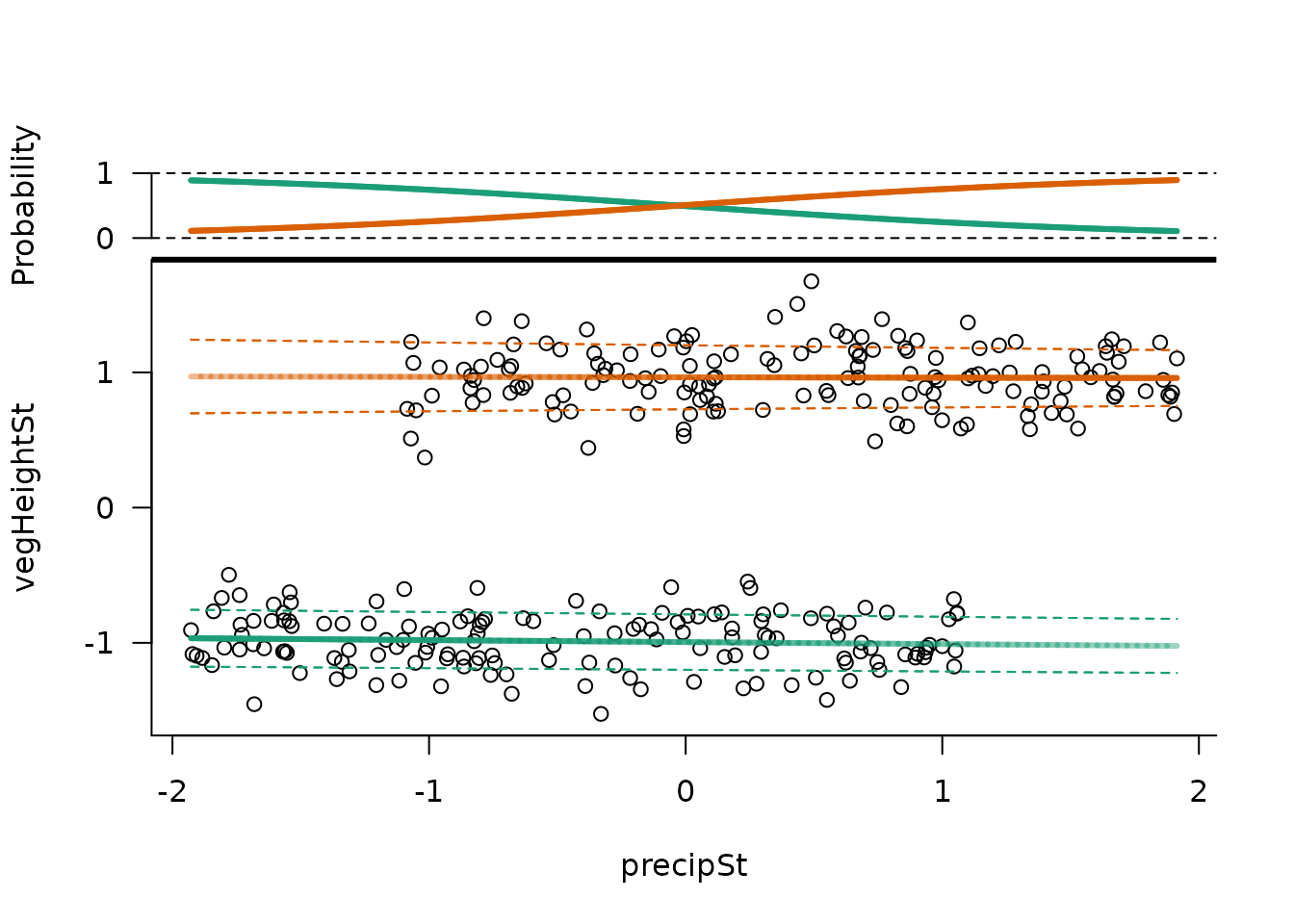

Model specifications

mixglm allows different predictors for individual components. For each sub-model (stateValModels / statePrecModels / stateProbModels), we can provide a list of formulas with each formula used for one component. This can be used e.g. to explore model behavior or test specific hypotheses.

statePrecModels <- list(~ precipSt, ~ 1) # precision of 2. component is constant

Priors can be specified using the setPriors argument. It takes a list of up to three named lists, one for each sub-model. We can specify priors for intercept parameters and priors for slope parameters. int1 denotes the intercept of the first component and int2 denotes intercept of all other components. Here we show several examples of setting priors:

# Full specification of priors
setPriors <- list(               
  stateVal = list(             # dnorm(mean, tau) parametrization is used
    int1 = "dnorm(0.0, 0.01)", #   by default, where sd = 1 / sqrt(tau)  
    int2 = "dgamma(1.0, 1.0)", # dgamma(shape, rate) parametrization is used
    pred = "dnorm(0.0, 0.01)"), 
  stateProb = list(
    int2 = "dnorm(0.0, sd = 10.0)",  # alternative parametrization can be used
    pred = "dnorm(0.0, 0.01)"),
  statePrec = list(
    int = "dnorm(0.0, 0.01)",
    pred = "dnorm(0.0, 0.01)"))

# Specification of priors for regression slope (effect of predictors on mean
#   value of each component). All unspecified priors are set to defaults. 
setPriors <- list(               
  stateVal = list(
    pred = "dnorm(0.0, 0.1)"))

# Specification of all intercept priors. All unspecified priors are set to 
#   defaults. 
setPriors <- list(               
  stateVal = list(             
    int1 = "dnorm(5.0, 1.0)",  
    int2 = "dbeta(1.0, 20.0)"),
  stateProb = list(             
    int2 = "dnorm(0.0, 0.1)"), 
  statePrec = list(            
    int = "dnorm(0.0, 0.1)"))

The mixglm() function has six arguments to control the MCMC run. Arguments mcmcIters, mcmcBurnin, mcmcChains, and mcmcThin can be used to set the number of iterations for each MCMC chain, the number of initial iterations to be discarded, the number of MCMC chains, and the thinning interval respectively. setSeed sets R’s random number seed. The argument setInit can be used to specify starting values for the sampler. This can be useful for exploration of parameter space or to ensure valid starting values. Initial values of a model can be accessed by mod$initialValues.

Results

In addition to the plot() function which visualizes individual components along a predictor, mixglm offers several other functions for accessing and plotting results.

Accessing results

Calling the model object (mod in our case) prints WAIC and posterior mean values for all parameters. These values can be accessed using the coef() function. For a more detailed overview, summary() function also provides the standard deviation, 2.5, 25, 75, and 97.5 percentiles of the posterior distribution for each parameter. Using the argument byChains = TRUE, we obtain this summary separately for each chain.

The summary() function has two more useful arguments. Intercepts for the mean values of components are in mixglm always modeled as a sum of all intercept parameters with the same or lower rank (in combination with positive priors for intercept parameters with rank > 1, this is to ensure identifiability of the model). Therefore, intercept parameters for the stateVal sub-model do not represent intercepts of individual components (but their cumulative sum does). To get intercepts of individual components, set parameter absInt = TRUE. Finally, the argument randomSample can be used to take random samples of parameters from their posterior distributions.

summary(mod, absInt = TRUE)
#> [[1]]
#>                           mean     sd    2.5%     25%     75%   97.5%
#> intercept_statePrec[1]  3.1693 0.1319  2.8972  3.0834  3.2639  3.4116
#> intercept_statePrec[2]  2.8808 0.1331  2.6087  2.7954  2.9721  3.1294
#> intercept_stateProb[1]      NA     NA  0.0000  0.0000  0.0000  0.0000
#> intercept_stateProb[2]  0.0292 0.1291 -0.2240 -0.0626  0.1205  0.2756
#> intercept_stateVal[1]  -0.9946 0.0185 -1.0291 -1.0074 -0.9819 -0.9558
#> intercept_stateVal[2]   0.9640 0.0228  0.9198  0.9485  0.9795  1.0087
#> precipSt_statePrec[1]   0.0269 0.1348 -0.2439 -0.0645  0.1174  0.2869
#> precipSt_statePrec[2]   0.1445 0.1427 -0.1329  0.0442  0.2389  0.4282
#> precipSt_stateProb[1]       NA     NA  0.0000  0.0000  0.0000  0.0000
#> precipSt_stateProb[2]   1.0937 0.1496  0.8054  0.9944  1.1942  1.3847
#> precipSt_stateVal[1]   -0.0148 0.0189 -0.0521 -0.0274 -0.0022  0.0220
#> precipSt_stateVal[2]   -0.0029 0.0222 -0.0466 -0.0180  0.0120  0.0403

Plotting results

mixglm has two functions to visualize the resulting mixture distributions. The function landscapeMixglm() shows a heatplot presentation of the fitted mixture with reddish colours denoting high probability density (in resilience modelling called the stability landscape). It plots the probability density scaled to range from 0 to 1 and highlights local maxima (suggesting stable states in resilience modelling; blue by default) and local minima (tipping points; red by default).

landscapeMixglm(mod, axes = FALSE, xlab = "Precipitation (mm/yr)", 
  ylab = "Vegetation height (cm)")
axis(1, labels = 1:3*500, at = st(1:3*500, precip))    # non-standardized 
axis(2, labels = 1:4*500, at = st(1:4*500, vegHeight)) #   values on axes

In the case there are multiple predictors, the argument form can be used to specify which predictor to visualize on the horizontal axis, and the argument otherPreds to specify values of predictors which are not visualized. Be aware that (as for ordinary multiple regression) for multiple predictors, observations (black points) are projected to the visualized plane and thus cannot be used to assess the fit of the model to the data.

Often the resulting mixture has small local minima or maxima which do not represent major peaks on the probability density function. If minima and maxima of the probability density are of interest (as in resilience modelling), it is useful to set a threshold and consider only major bumps in the probability density function as actual minima/maxima. The argument threshold can be used to denote only such minima/maxima which differ in the scaled probability density by at least specified value.

landscapeMixglm(mod, threshold = 0.3)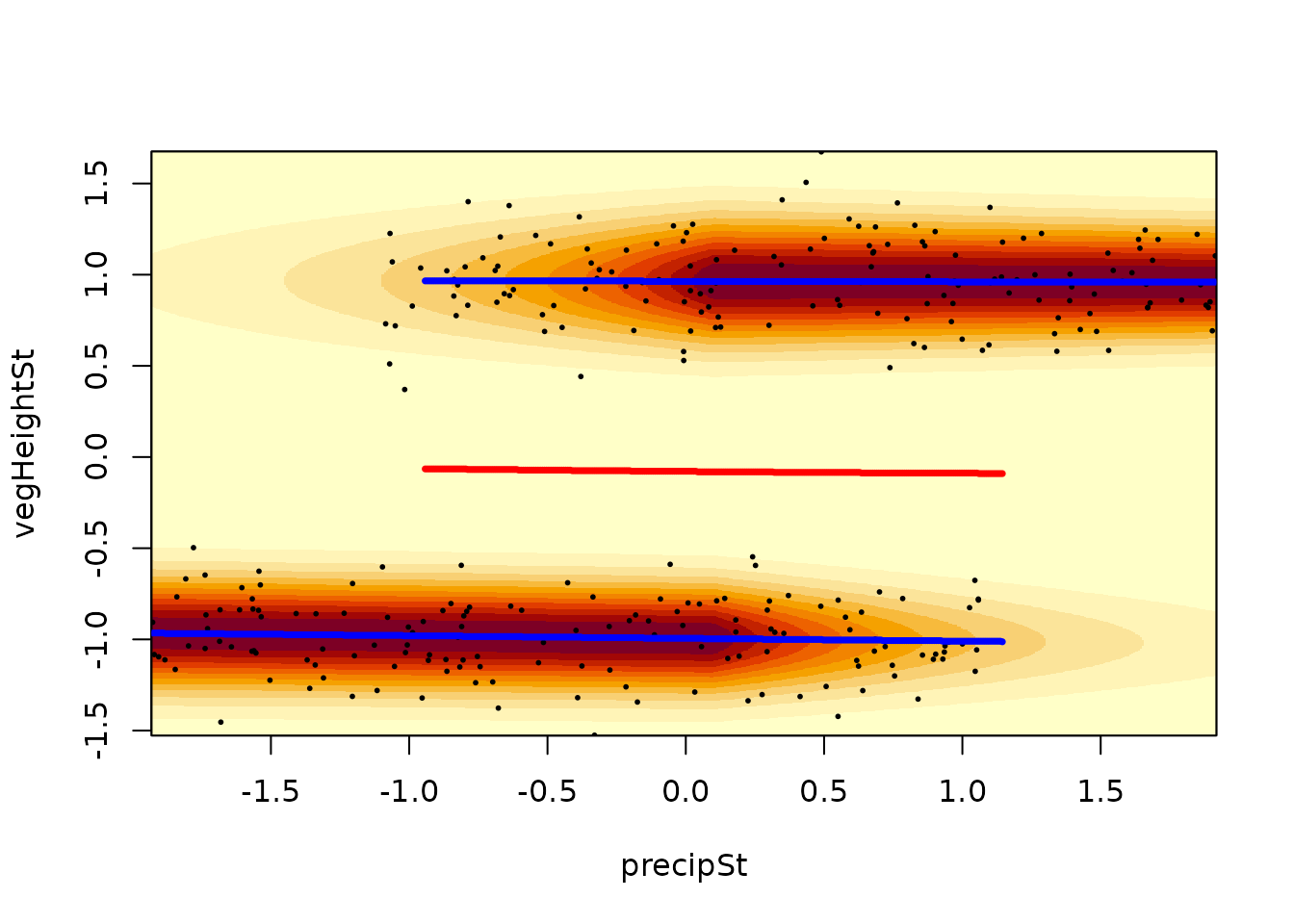

The argument randomSample of the landscapeMixglm() function can be used to assess uncertainty in the results. It specifies how many random samples from the posterior distribution should be taken. For each of these samples, the probability density of the mixture is evaluated and the standard deviation of these evaluations is plotted alongside the local minima and maxima for each of them. These computations can take some time, thus we illustrate it here using just 3 samples:

landscapeMixglm(mod, threshold = 0.3, randomSample = 3)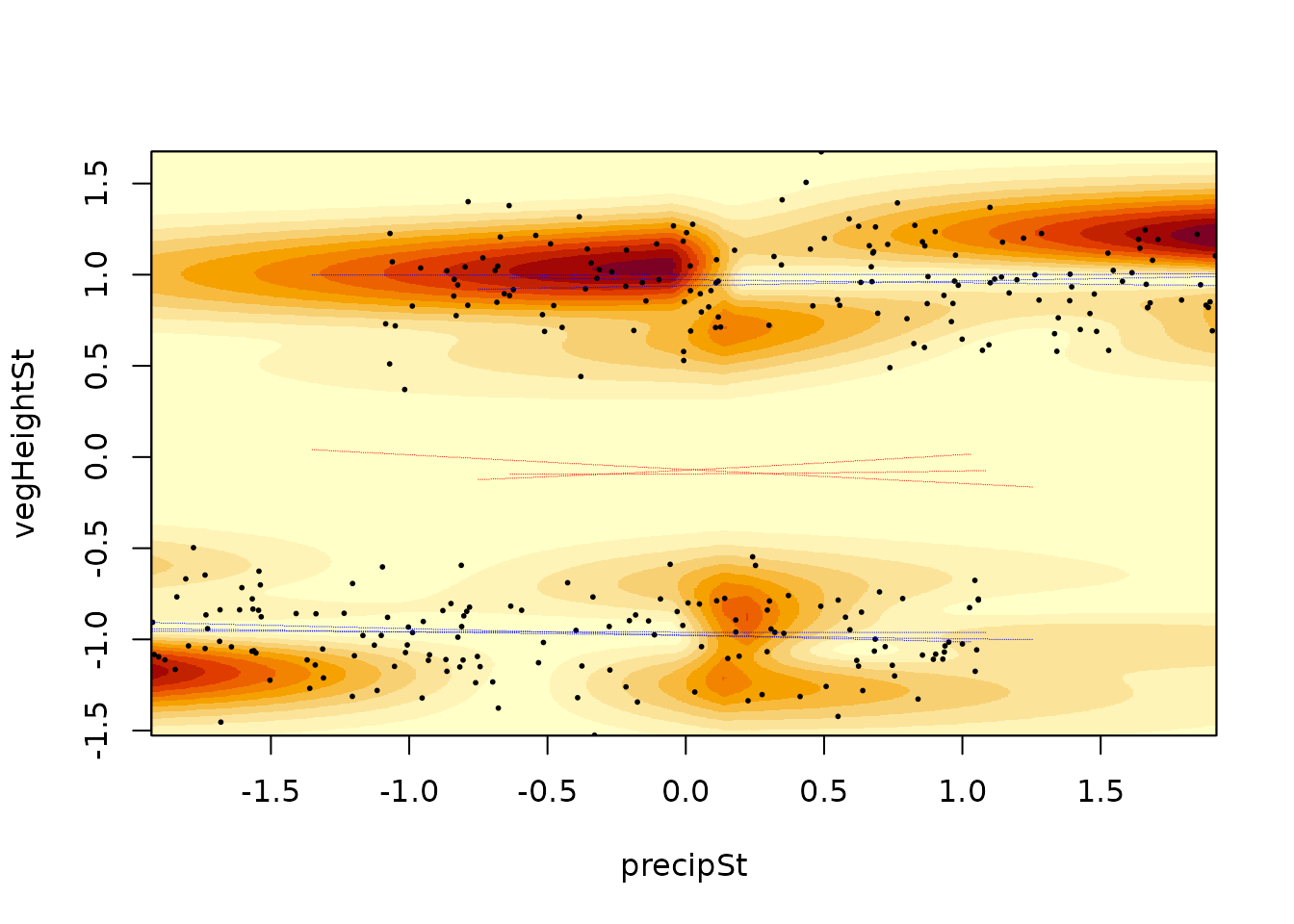

The second plotting function is sliceMixglm(). It can be understood as a vertical slice through the plot from the landscapeMixglm() or plot() functions. It shows the probability density for a given predictor value (argument value; in resilience modelling called stability curve). It also highlights the mean of each mixture component (by default using the same colours as the plot() function). As in the plot() function, sliceMixglm() has an argument byChains (which is by default TRUE) showing the probability density and mean of mixtures for each chain (thus highlighting improper convergence of chains).

sliceMixglm(mod, value = 0.5) # precipSt == 0.5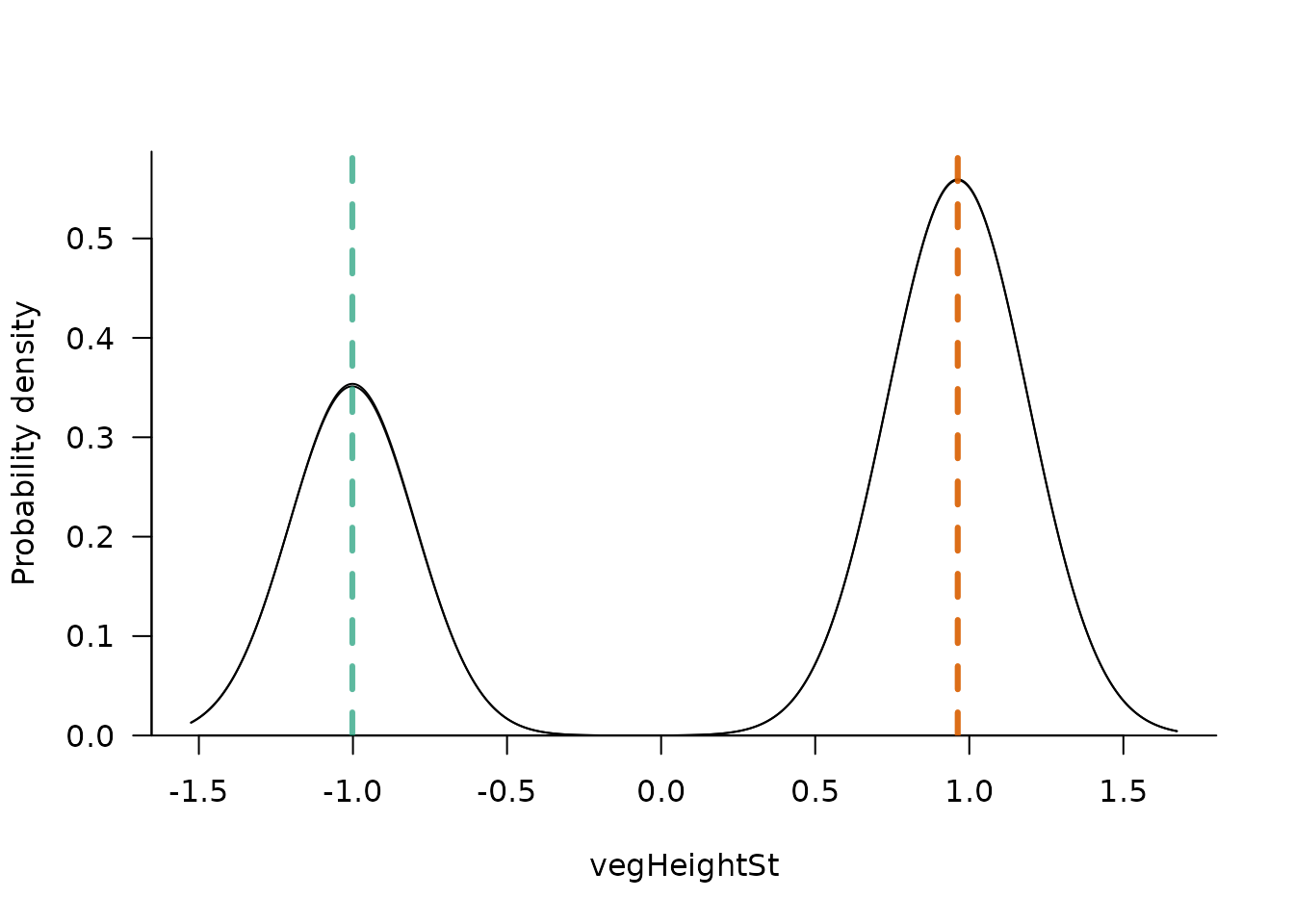

The argument addEcos can be used to include observations with similar predictor values (differing up to ecosTol, by default 0.1).

sliceMixglm(mod, value = 0.5, addEcos = TRUE, ecosTol = 0.3)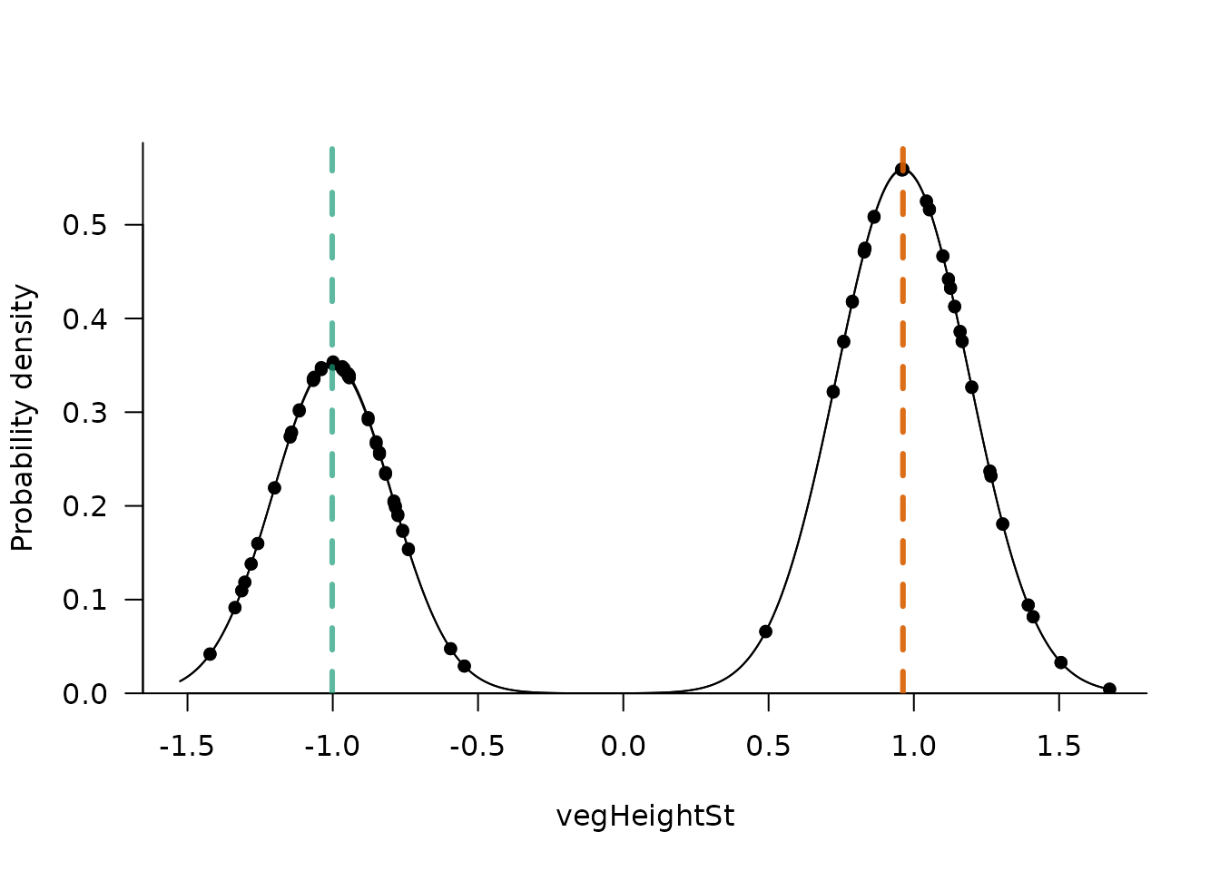

The argument randomSample is used instead of the posterior mean to take and plot random samples from the posterior distributions of parameters.

Predictions

To predict the scaled probability density of the mixture for specific predictor values or to obtain local minima/maxima for those values, mixglm has the functionpredict(). By providing predictor values as a named data.frame to the newdata argument, we get a list with a probCurves item which stores the scaled probability density for each predictor value along the response variable (response variable values are stored in item sampledResp). Item tipStable provides a data.frame for each provided predictor value of local minima (state == 0) and maxima (state == 1) of the probability density. Those which pass a user defined threshold (specified by the threshold argument) are marked as catSt == 1. The scaled probability density of these local minima and maxima and their response values are also provided.

pred <- predict(mod, newdata = data.frame(precipSt = c(-1.5,0,1.5), 
  vegHeightSt = c(1, 1, 1)), threshold = 0.3)

# we can e.g. produce plots similar to sliceMixglm()
plot(pred$probCurves$X1 ~ pred$sampledResp, type = "l")

# we add highlighting of local minima/maxima and if they reach the threshold
tipStable1 <- pred$tipStable[[1]]
cols <- c("red", "blue")
points(tipStable1$resp, tipStable1$probDens, col = cols[tipStable1$state + 1],
 pch = c(1, 16)[tipStable1$catSt + 1])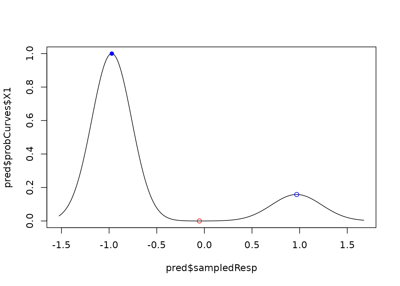

Resilience measures

The function predict() also allows calculation of several resilience measures. Potential energy (potentEn) is a scaled probability density for each observation. distToState is distance to the closest stable state (local maxima of probability density) taking threshold into account. Distance is in units of the response variable and can be understood as a vertical distance of an observation to a blue line in the landscapeMixglm() figure. For observations with tipping points on their stability curve (local minima of probability density), distance to closest tipping point (distToTip) and potential depth (potentialDepth) is provided. Potential depth is the difference in potential energy between an observation and the closest tipping point.

# prediction for the original (modeled) data can be done by omitting the 
#   argument `newdata`
predOrig <- predict(mod, threshold = 0.3) 
par(mfrow = c(2,2))                       
plot(dat$precip, dat$vegHeight, cex = predOrig$obsDat$potentEn * 2, 
  main = "Potential energy")
plot(dat$precip, dat$vegHeight, cex = predOrig$obsDat$distToState * 4, 
  main = "Distance to stable state")
plot(dat$precip, dat$vegHeight, cex = predOrig$obsDat$distToTip, 
  main = "Distance to tipping point")
plot(dat$precip, dat$vegHeight, cex = predOrig$obsDat$potentialDepth * 1.5, 
  main = "Potential depth")

References

↑ Dakos, V., Kéfi, S., 2022. Ecological resilience: what to measure and how. Environmental Research Letters 17: 043003. doi.org/10.1088/1748-9326/ac5767

↑ Klimeš, A., Chipperfield, J., Töpper, Macias-Fauria, J., Spiegel, M., Vandvik, V., Velle, L. G., Seddon, A. [mixglm]: A tool for modelling ecosystem resilience. bioRxiv. doi.org/10.1101/2024.03.23.586419

↑ McLachlan, G., Peel, D., 2000. Finite Mixture Models. A Wiley-Interscience Publication. John Wiley & Sons, Inc. ISBN 0-471-00626-2

↑ Watanabe, S. 2013. A widely applicable bayesian information criterion. Journal of Machine Learning Research 14: 867–897. Link

Mixture models with mixglm

Contents